Page MenuHomePhabricator

Google-referred desktop traffic decline vs overall desktop traffic decline
Closed, DeclinedPublic4 Estimated Story Points

Description

This was a question posed by @DarTar at today's (October) Monthly Metrics Meeting during the Q&A:

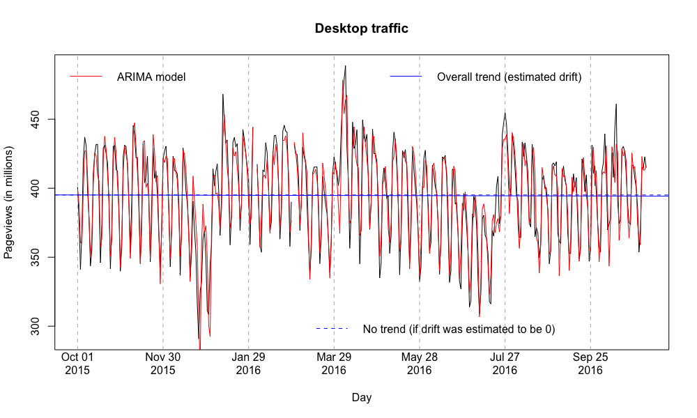
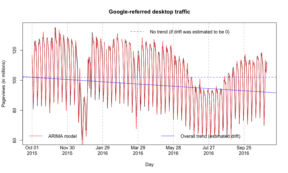
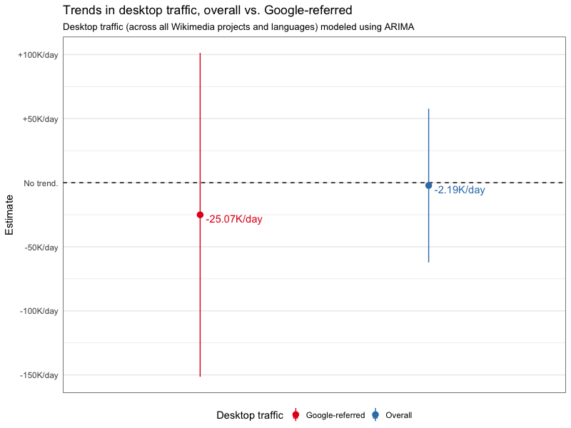
I was curious about the rate at which search engine traffic is declining, not just the absolute numbers. In other words: is Google referred traffic declining at the same rate as the overall decline of desktop traffic? Or faster? Past longitudinal data suggested it was dropping faster.

Event Timeline

Pinging @MelodyKramer who might be interested in following along and/or using this ticket for reference later :)

debt triaged this task as Medium priority.Oct 27 2016, 8:17 PM
mpopov added a subscriber: chelsyx.

I'm not the topmost expert in ARIMA modeling and interpretation, especially when there's differencing involved (although I think units remain the same???), but I gave this my best shot. If @chelsyx or anyone else wants to point out my mistakes, that would be awesome and greatly appreciated. Basically what we're seeing is, I think, a faster decline in Google-referred desktop traffic compared to decline in desktop traffic overall because after adjusting for seasonality and auto-correlation, we are seeing a steeper negative trend. (Although, like I said, the differencing of Google-referred desktop traffic due in order to get stationarity means that the interpretation of the drift coefficient may not be 100% correct.) Compare:

desktop.png (600×1 px, 178 KB)

vs.

google.png (600×1 px, 207 KB)

Here are the estimates of the drift (the slope of the trend line) with +1/-1 standard errors bounds:

drift.png (600×800 px, 42 KB)

Appendix (Code)

Prereqs

install.packages(c("devtools", "tidyverse", "forecast"))
devtools::install_github(c(
  "hadley/ggplot2",
  "wikimedia/wikimedia-discovery-polloi"
), dependencies = TRUE)

Data

library(tidyverse)

traffic <- polloi::read_dataset(path = "external_traffic/referer_data.tsv", col_types = "Dlccci")
pageviews <- traffic %>%
  filter(access_method == "desktop") %>%
  group_by(date) %>%
  summarize(
    total_pageviews = sum(pageviews),
    google_referred_pageviews = sum(pageviews[referer_class == "external (search engine)" & search_engine == "Google"])
  )

# Detect missing days and impute missing data:
# sum(!seq(min(pageviews$date), max(pageviews$date), "day") %in% pageviews$date)
tmp <- data.frame(date = seq(min(pageviews$date), max(pageviews$date), "day"))
tmp$time <- 1:nrow(tmp)

pv_total <- pageviews %>%
  right_join(tmp, "date")

ARIMA Modeling

library(forecast)

fit_total <- Arima(pv_total$total_pageviews/1e6,
                   include.mean = TRUE,
                   include.drift = TRUE,
                   order = c(1, 0, 1),
                   seasonal = list(order = c(1, 0, 1), period = 7),
                   method = "ML")

fit_google <- Arima(pv_total$google_referred_pageviews/1e6,
                    include.mean = TRUE,
                    include.drift = TRUE,
                    order = c(3, 1, 3),
                    seasonal = list(order = c(1, 0, 0), period = 7),
                    method = "ML")

Visualization

Time Series

plot(pv_total$time, pv_total$total_pageviews/1e6, type = "l",
     xlab = "Day", ylab = "Pageviews (in millions)",
     main = "Desktop traffic", xaxt = "n")
abline(v = seq(1, nrow(pv_total), 60), lty = "dashed", col = "gray70")
axis(side = 1, at = seq(1, nrow(pv_total), 60), tick = FALSE,
     labels = as.character(pv_total$date[seq(1, nrow(pv_total), 60)], "%b %d\n%Y"))
lines(fitted(fit_total), col = "red")
abline(h = coefficients(fit_total)["intercept"],
       col = "blue", lty = "dashed")
abline(a = coefficients(fit_total)["intercept"],
       b = coefficients(fit_total)["drift"],
       col = "blue")
legend("topleft", "ARIMA model", col = "red", lty = "solid", lwd = 1, bty = "n")
legend("bottomright", "No trend (if drift was estimated to be 0)", col = "blue", lty = "dashed", lwd = 1, bty = "n")
legend("topright", "Overall trend (estimated drift)", col = "blue", lty = "solid", lwd = 1, bty = "n")

plot(pv_total$time, pv_total$google_referred_pageviews/1e6, type = "l",
     xlab = "Day", ylab = "Pageviews (in millions)",
     main = "Google-referred desktop traffic", xaxt = "n")
abline(v = seq(1, nrow(pv_total), 60), lty = "dashed", col = "gray70")
axis(side = 1, at = seq(1, nrow(pv_total), 60), tick = FALSE,
     labels = as.character(pv_total$date[seq(1, nrow(pv_total), 60)], "%b %d\n%Y"))
lines(fitted(fit_google), col = "red")
# differencing because we don't have a stationary TS, which means we won't have an intercept coef
# coefficients(fit_total)["intercept"] is close to mean(pv_total$total_pageviews/1e6)
# so let's use that as the faux intercept
abline(h = mean(pv_total$google_referred_pageviews/1e6, na.rm = TRUE),
       col = "blue", lty = "dashed")
abline(a = mean(pv_total$google_referred_pageviews/1e6, na.rm = TRUE),
       b = coefficients(fit_google)["drift"],
       col = "blue")
legend("bottomleft", "ARIMA model", col = "red", lty = "solid", lwd = 1, bty = "n")
legend("topright", "No trend (if drift was estimated to be 0)", col = "blue", lty = "dashed", lwd = 1, bty = "n")
legend("bottomright", "Overall trend (estimated drift)", col = "blue", lty = "solid", lwd = 1, bty = "n")

Drift Estimate & Standard Error Bounds

list(
  `Overall` = fit_total,
  `Google-referred` = fit_google
) %>%
  lapply(broom::tidy) %>%
  bind_rows(.id = "Desktop traffic") %>%
  filter(term == "drift") %>%
  ggplot(aes(x = 1, y = estimate,
             ymin = estimate - std.error,
             ymax = estimate + std.error,
             color = `Desktop traffic`)) +
  geom_hline(aes(yintercept = 0), linetype = "dashed") +
  geom_pointrange(position = position_dodge(width = 1)) +
  scale_color_brewer(palette = "Set1") +
  scale_y_continuous(labels = function(x) {
    labels <- paste0(ifelse(sign(x) > 0, "+", "-"), polloi::compress(abs(x) * 1e6), "/day")
    labels[labels == "-0K/day"] <- "No trend."
    return(labels)
  }) +
  geom_text(aes(label = paste0("  ", ifelse(sign(estimate) > 0, "+", "-"), polloi::compress(abs(estimate) * 1e6), "/day"),
                vjust = "top", hjust = "left"),
            position = position_dodge(width = 1)) +
  labs(x = NULL, y = "Estimate",
       title = "Trends in desktop traffic, overall vs. Google-referred",
       subtitle = "Desktop traffic (across all Wikimedia projects and languages) modeled using ARIMA") +
  theme_minimal() +
  theme(legend.position = "bottom",
        panel.grid.major.x = element_blank(),
        panel.grid.minor.x = element_blank(),
        axis.ticks.x = element_blank(),
        axis.text.x = element_blank(),
        strip.background = element_rect(fill = "gray90"),
        panel.border = element_rect(color = "gray30", fill = NA))

@HJiang-WMF @Tbayer @chelsyx When you get a chance, could you please check my work on this? Time series analysis is my weakest area and I couldn't find a lot of literature on answering questions like this :(

I don't think I'm dealing with the drift term from the differenced time series correctly, but I have no idea how to transform it into a non-differenced scale. (If that makes sense.)

@mpopov I cannot reproduce your results with the code above: for fit_total, I got drift = 0.003480768; for fit_google, I got drift=-0.003127302. From your result above, trend=0 is within +1/-1 standard errors, which means drift is not significant and there are no trend in both series.

Also, I'm confused with the result of Arima. From my understanding, when d=0 and the model fit well, there should be no trend in the series, which means drift=0. When d=1, drift is the slope and is also an estimate of the mean of the differenced data.

I'm not an expert in time series either, so any comments are greatly appreciated!!! :)

Reference: http://robjhyndman.com/hyndsight/arima-trends/

@mpopov I tried 3 times to reproduce your results with your code, but each time the drift and fit_google actually match up with results from @chelsyx. Also, from what I have dealt with time series, there are different non-stationary behaviors to check for before differencing: trends, cycles, random-walks, disturbance, etc., and it helps a lot to try different stationarizing techniques, depending on what kind of non-stationary behavior the TS exhibits. De-trending, de-differencing(the key stats are constant over periods or seasons), etc. could be helpful in this context

Very interesting work! A few notes:

  • If I'm reading this correctly, the source data (referer_data.tsv) does not filter out spiders (via agent_type = 'user'). I guess this does not matter when counting Google-referred pageviews, but for the overall desktop traffic it makes a huge difference and should be corrected.
  • Also, looking at the large spike from July on in the first graph above, it looks like overall desktop pageview numbers used here have not yet been corrected for T141506 (an issue which artificially inflated desktop pageviews by about 20% during that time).
  • We know that besides the weekly patterns (which the ARIMA models here appear to do a good job of capturing), our traffic also exhibits a strong yearly seasonality, which the present analysis does not and can not account for because it is only based on about a year's worth of data. The received wisdom (also from eyeballing the linked chart) is that overall traffic has generally been lower in the northern summer months. These happen to fall into the later part of the timespan analyzed here. In other words, the decline observed above is likely at least partly due to yearly seasonality. Even the relative difference between the trend of overall desktop views and Google-referred views could be entirely caused by yearly seasonality, if the latter happen to drop more every summer than the overall views. So I'm wondering what's the best way to draw general conclusions here.

@chelsyx @HJiang-WMF @Tbayer Thank you all so much for the feedback and suggestions!

@chelsyx @HJiang-WMF The reason for the irreproducibility is that the dataset grows every day, so running the same code several days after the original post should yield only slightly different coefficient estimates.

@Tbayer Thanks for pointing out the inflation! I'm not sure how to correct that (since we don't have access to raw July data for a recount) other than maybe introduce an indicator covariate into the ARIMA model that is 1 during the period of inflation and 0 otherwise. Good call on agent type for desktop traffic. Not sure what we can do about that at this stage :\

Tilman makes an excellent point about the yearly seasonality (and actual literal seasons). It may be too hard to draw general conclusions until we have two full years of data?

...

@Tbayer Thanks for pointing out the inflation! I'm not sure how to correct that (since we don't have access to raw July data for a recount) other than maybe introduce an indicator covariate into the ARIMA model that is 1 during the period of inflation and 0 otherwise. Good call on agent type for desktop traffic. Not sure what we can do about that at this stage :\

Oh, we can address both (the July/August inflation and spiders in general) by backfilling the data from the pageview_hourly table, where the information is still preserved - cf. the query I linked above.

Tilman makes an excellent point about the yearly seasonality (and actual literal seasons). It may be too hard to draw general conclusions until we have two full years of data?

BTW we actually have (sampled) pageview data back to 2013, see here. I have been using it to analyze the longer term trends in overall pageviews (which involves some adjustments for changes to the definition over time). If it is of interest, I can provide such a time series for daily *desktop* pageviews too.
That table also contains a "referer" field where Google referrals are marked separately, but I don't know the definition or whether it is compatible to the one used here. It seems that it was used (or maybe not - unfortunately some of the underlying code seems to have been removed from Github) in Oliver's August 2015 analysis of Google-referred pageviews (T108895), which may be worth comparing anyway. E.g. rather than modeling overall views and Google-referred views separately and then comparing the trends, it analyzed their ratio (the proportion of Google-referred views), which may simplify things in some aspects.

debt subscribed.

Moving to the backlog for now, until we have more time to work on it.

@debt, @mpopov: I am working on deleting raw logs, I cc-ed Mikhail but haven't received an answer yet. Could one of you please contact me to go over what's being deleted and whether you need it or not? Based on what Dario says, those logs are your only data source for the work on this ticket.

For context: scanning the conversation on this task, people brought up valid concerns regarding the lack of longitudinal data to filter annual seasonality. As far as I know, the sampled logs have been used in the past by @Ironholds to produce longer time series based on an R-implementation of the PV definition. cc @Erik_Zachte

As an update, Mikhail gave the ok to delete these logs on the email thread, so the historical ones are deleted. Happy to help people set up this kind of analysis and run it on an on-going basis. We do have some logs we backed up for legal if people are interested in looking at a bit older data from around 2015.

Declining this ticket - I think that @Tbayer and others answered the questions that @DarTar asked. :) Please re-open and add comments if it needs to be further investigated.

Declining this ticket - I think that @Tbayer and others answered the questions that @DarTar asked. :) Please re-open and add comments if it needs to be further investigated.

Thanks ;) but I don't think I answered any of those questions. To the contrary, I would have been quite interested in the answers myself. (And not just I - the influence of Google referrals on Wikipedia readership, and how it has been developing over time, has been an important discussion topic both in the Wikimedia movement and among external observers for many years.)
That said, personally I understand the team's need to limit unplanned work, and also now that we have deleted the data that would have been most suitable to answer such questions, it probably doesn't make much sense to pursue the present analysis further.